Simple Finite Impulse Response Notch Filter

Pieter P

This is an example on how to design a very simple FIR notch filter in the digital domain, that can be used to filter out 50/60 Hz mains noise, for example.
It is a very simple filter, so the frequency response is not great, but it might be all you need. It's only second order, finite impulse response, so very fast and always stable, and has linear phase.

Zero Placement

To achieve notch characteristics, we'll just place a single complex pair of zeros on the unit circle. Let's say we have a sample frequency of $360 Hz$ and we want to filter out $50 Hz$ noise.
We'll first calculate the normalized frequency $ω_{c, d}$ : $\begin{aligned} f_{s} & = 360 Hz \\ f_{c} & = 50 Hz \\ ω_{c} & = 2 π f_{c} \approx 314.2 rad s^{- 1} \\ ω_{c, d} & = \frac{ω_{c}}{f_{s}} \approx 0.8727 \frac{rad}{sample} \end{aligned}$ We know that the frequency response $H (ω)$ of a digital filter is just the transfer function $H (z)$ evaluated along the unit circle $z = e^{j ω}$ . In other words, we just need a transfer function that is zero when the frequency equals $ω_{c, d}$ , or when $z = e^{j ω_{c, d}}$ . Because the transer function must have real coefficients, the complex conjugate will be a zero as well: $z = e^{- j ω_{c, d}}$ . $H^{'} (z) = (z - e^{j ω_{c, d}}) (z - e^{- j ω_{c, d}})$ We can further simplify this function by expanding it, and using the identity $\cos (θ) = \frac{e^{j θ} + e^{- j θ}}{2}$ : $\begin{aligned} H^{'} (z) & = z^{2} - z (e^{j ω_{c, d}} + e^{- j ω_{c, d}}) + e^{j ω_{c, d}} e^{- j ω_{c, d}} \\ = z^{2} - 2 \cos (ω_{c, d}) z + 1 \end{aligned}$

A Proper Transfer Function

The transfer functions of all physical processes are proper. This means that the degree of the numerator is not larger than the degree of the denominator.
This is clearly not the case for $H^{'} (z)$ (the degree of the numerator is 2 and the degree of the denominator is 0).

The solution is simple: we'll just add two poles in $z = 0$ . This won't affect the frequency response. $H (z) = \frac{H^{'} (z)}{z^{2}} = \frac{z^{2} - 2 \cos (ω_{c, d}) z + 1}{z^{2}} = 1 - 2 \cos (ω_{c, d}) z^{- 1} + z^{- 2}$

Normalization

If we want a filter with a unit DC gain ( $H (1) = 1$ ), we can just normalize the transfer function: $H_{n} (z) = \frac{H (z)}{H (1)} = \frac{1 - 2 \cos (ω_{c, d}) z^{- 1} + z^{- 2}}{2 - 2 \cos (ω_{c, d})}$

Numerical Result

Finally, we can just plug in the value of $ω_{c, d}$ : $H_{n} (z) \approx \frac{1 - 1.286 z^{- 1} + z^{- 2}}{0.7144} = 1.400 - 1.800 z^{- 1} + 1.400 z^{- 2}$

Bode Plot & Zero Map

Let's take a quick look at the bode plot and the locations of the zeros. The Python code to generate the Bode plot can be found below. You can clearly see the expected linear phase of a FIR filter, with a 180 phase jump when the frequency crosses the zero. The notch itself is not at all narrow. If you want a narrower notch, you could a higher FIR order, or place some poles close to the unit circle to cancel the effect of the zero.

The magnitude of the transfer function in function of the complex variable $z$ looks like this.

Image source code

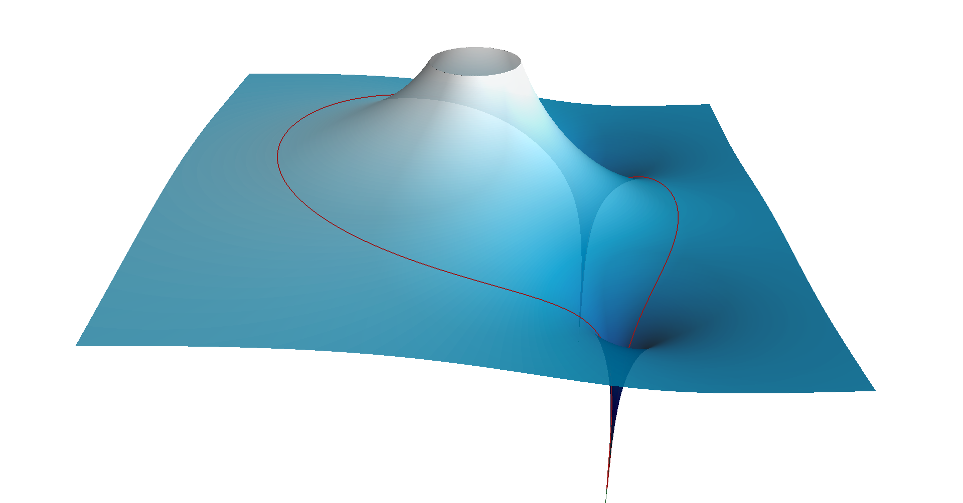
The red curve is the image of the unit circle in the complex plane ( $| z | = 1$ ). The vertical axis uses a logarithmic scale, just like on the Bode plot above. The elevation of the surface along the top half of the unit circle corresponds to magnitude value on the Bode plot along the horizontal axis.
Note the two zeros on the unit circle that cause the magnitude to go to $- \infty dB$ for these frequencies, as well as the two poles in the origin that cause the high spike.

#!/usr/bin/env python3

from scipy.signal import butter, freqz 
import matplotlib.pyplot as plt
from math import pi, cos
import numpy as np

f_s = 360    # Sample frequency in Hz
f_c = 50     # Notch frequency in Hz

omega_c = 2 * pi * f_c       # Notch angular frequency
omega_c_d = omega_c / f_s    # Normalized notch frequency (digital)

h_0 = 2 - 2 * cos(omega_c_d)
b = np.array((1, -2 * cos(omega_c_d), 1))   # Calculate coefficients
b /= h_0                                    # Normalize
a = 1
print("a =", a)                      # Print the coefficients
print("b =", b)

w, h = freqz(b, a)                   # Calculate the frequency response
w *= f_s / (2 * pi)                  # Convert from rad/sample to Hz

plt.subplot(2, 1, 1)                 # Plot the amplitude response
plt.suptitle('Bode Plot')            
plt.plot(w, 20 * np.log10(abs(h)))   # Convert to dB
plt.ylabel('Magnitude [dB]')
plt.xlim(0, f_s / 2)
plt.ylim(-60, 20)
plt.axvline(f_c, color='red')

plt.subplot(2, 1, 2)                 # Plot the phase response
plt.plot(w, 180 * np.angle(h) / pi)  # Convert argument to degrees
plt.xlabel('Frequency [Hz]')
plt.ylabel('Phase [°]')
plt.xlim(0, f_s / 2)
plt.ylim(-90, 135)
plt.yticks([-90, -45, 0, 45, 90, 135])
plt.axvline(f_c, color='red')
plt.show()