Exponential Moving Average
Pieter PDifference equation
The difference equation of an exponential moving average filter is very simple:
The filter is called 'exponential', because the weighting factor of previous inputs decreases exponentially.
This can be easily demonstrated by substituting the previous outputs:
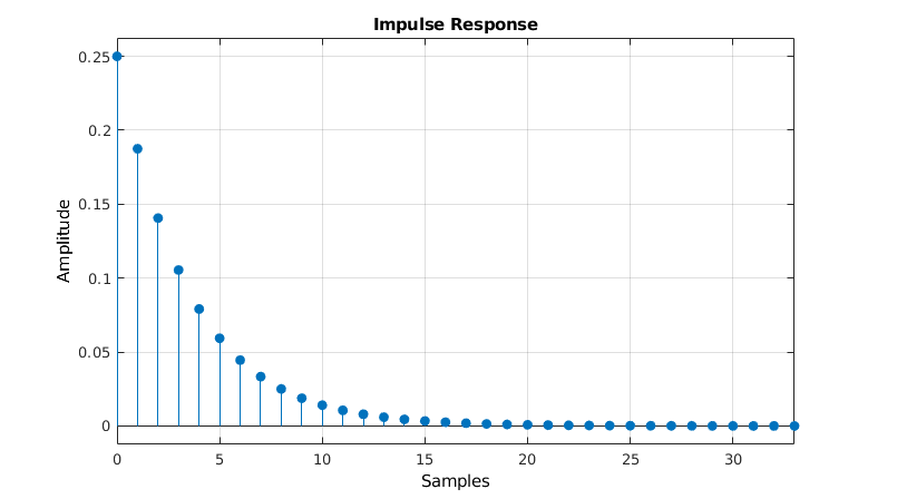
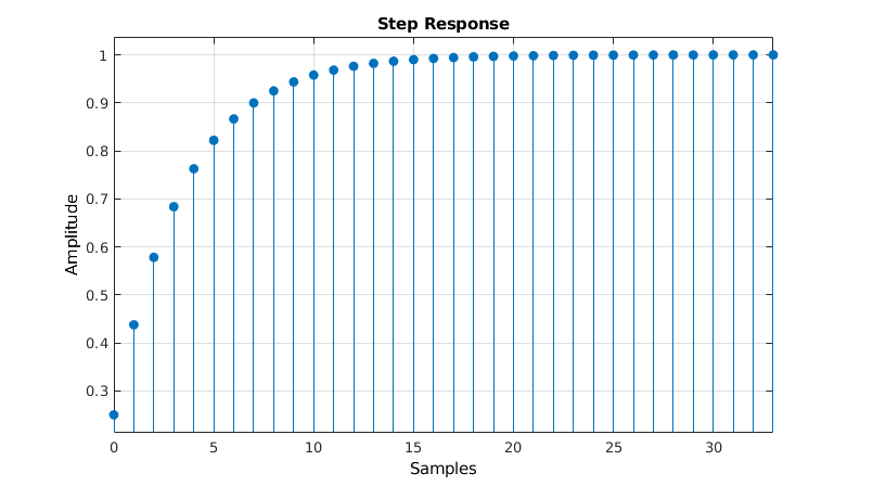
Impulse and step response
From the previous equation, we can now easily calculate the impulse and step response.
The impulse response is the output of the filter when a Kronecker delta function is applied to the input.
Recall the definition of the Kronecker delta:
The step response is the output of the filter when a Heaviside step function is applied to the input.
The Heaviside step function is defined as
Transfer function
The output of discrete-time linear time-invariant (DTLTI) systems, of which the EMA is an example, can be expressed as the convolution of the input with the impulse response. In other words, the impulse response describes the behavior of the system, for all possible inputs.
To prove the previous statement, we'll start with the following trivial property:
any signal
You can also interpret this as the signal being made up of a sum of infinitely many scaled and shifted Kronecker
delta functions.
Let
Analysis of such systems is usually easier in the Z-domain, in which the convolution is reduced to a simple
product.
The (unilateral) Z-transform is defined as:
Let's calculate the transfer function of the EMA.
We can use one of two approaches: use the difference equation and use some of
the properties of the Z-transform to calculate
Using the difference equation
All you have to do is apply the time shifting property of the Z transform:
Using the impulse response
Poles and zeros
In these expressions,
There are a couple of interesting values for
The poles and zeros determine the overall effect of the transfer function,
so pole-zero plots are a very useful tool when describing filters.
This is the pole-zero plot of the same example EMA as before, with 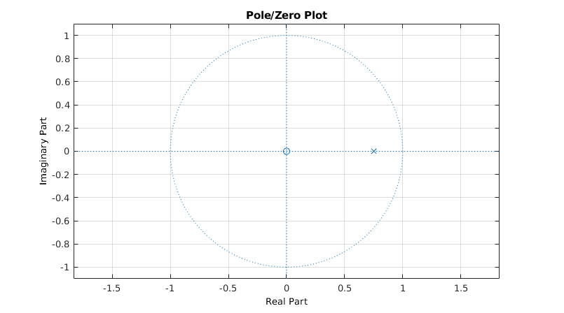 The zero in the origin is indicated by an O, and the pole at
Frequency response
An important property of discrete-time linear time-invariant systems is that it preserves the pulsatance (angular
frequency) of sinusoidal signals, only the phase shift and the amplitude are altered.
In other words, sines and cosines are eigenfunctions of DTLTI systems.
This makes it relatively easy to express the frequency response (sometimes called magnitude response) of a filter.
We're interested in the spectrum of frequencies that a signal contains, so it makes sense to decompose it as a sum
of sines and cosines. That's exactly what the discrete-time Fourier transform does:
The frequency response of the filter describes how the spectrum of a signal is altered when it passes
through the filter. It relates the spectrum of the output signal
We can now plot the filter's gain in function of the frequency. These plots often use a logarithmic scale, to
show the gain in decibels. In order to calculate the power gain, the amplitude is squared.
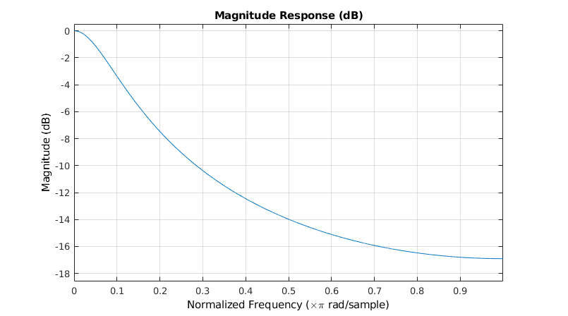 You can clearly see the low-pass behavior of the EMA: low frequencies have a near-unit gain, and high frequencies
are attenuated.
You can clearly see the low-pass behavior of the EMA: low frequencies have a near-unit gain, and high frequencies
are attenuated.
To get a better understanding of where this curve comes from, we can plot the entire 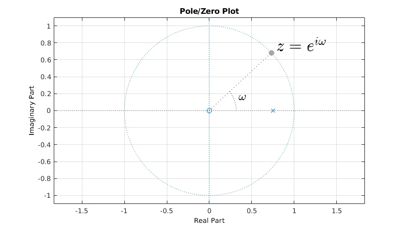
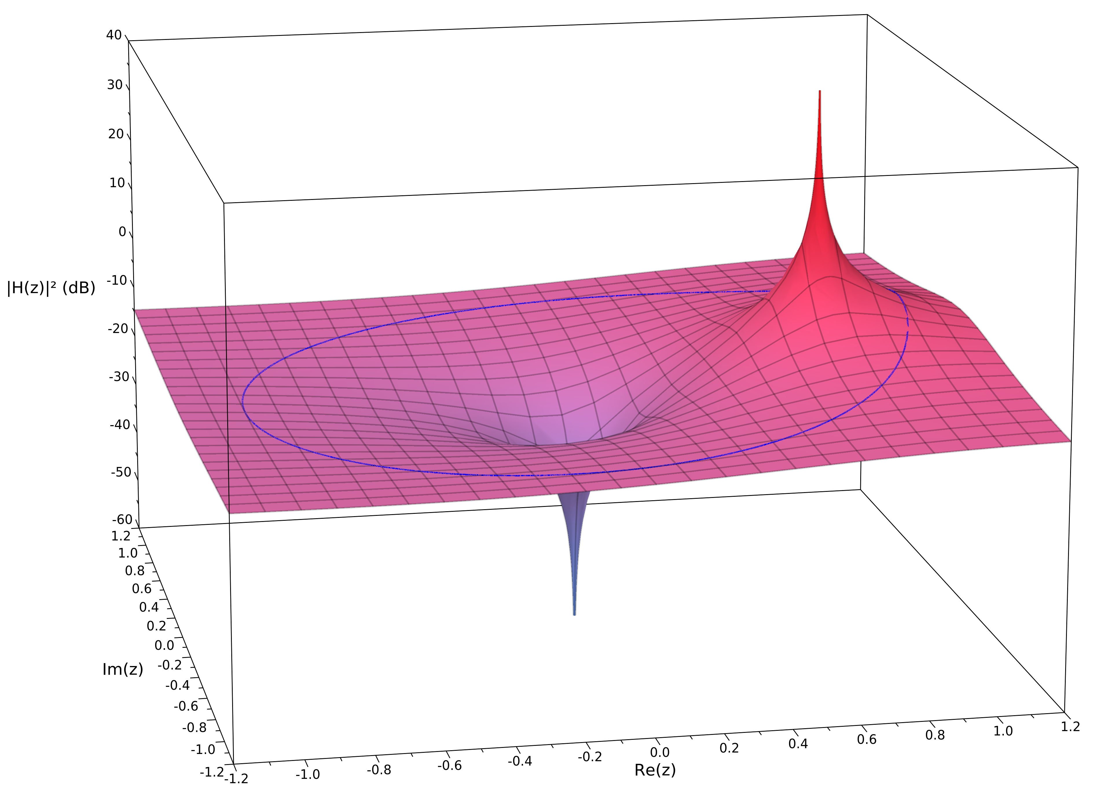 The image of the unit circle is shown in blue. Notice that this is the same curve as the blue curve in the
magnitude response graph above:
close to 0 when
The image of the unit circle is shown in blue. Notice that this is the same curve as the blue curve in the
magnitude response graph above:
close to 0 when
You can clearly see the effect of the pole at
Cutoff frequency
The cutoff frequency is defined as the frequency of the half-power point, where the power gain is a half. It's
often called the
To find it, just solve the following equation:
For example, if
To convert it to a frequency in Hertz, you can multiply
For example, if the sample frequency is
Plotting the frequency response in Python
We can use the SciPy and Matplotlib modules to plot the frequency response in Python.
The SciPy freqz function expects the transfer function coefficients in the form
In the case of the exponential moving average filter, the transfer function is

from scipy.signal import freqzimport matplotlib.pyplot as pltfrom math import pi, acosimport numpy as npalpha = 0.25b = np.array(alpha)a = np.array((1, alpha - 1))print("b =", b) # Print the coefficientsprint("a =", a)x = (alpha**2 + 2*alpha - 2) / (2*alpha - 2)w_c = acos(x) # Calculate the cut-off frequencyw, h = freqz(b, a) # Calculate the frequency responseplt.subplot(2, 1, 1) # Plot the amplitude responseplt.suptitle('Bode Plot')plt.plot(w, 20 * np.log10(abs(h))) # Convert to dBplt.ylabel('Magnitude [dB]')plt.xlim(0, pi)plt.ylim(-18, 1)plt.axvline(w_c, color='red')plt.axhline(-3, linewidth=0.8, color='black', linestyle=':')plt.subplot(2, 1, 2) # Plot the phase responseplt.plot(w, 180 * np.angle(h) / pi) # Convert argument to degreesplt.xlabel('Frequency [rad/sample]')plt.ylabel('Phase [°]')plt.xlim(0, pi)plt.ylim(-90, 90)plt.yticks([-90, -45, 0, 45, 90])plt.axvline(w_c, color='red')plt.show()
