Simple Moving Average

Difference equation

The difference equation of the Simple Moving Average filter is derived from the mathematical definition of the average of $N$ values: the sum of the values divided by the number of values. $$y[n]=\frac{1}{N}\sum _{i=0}^{N-1}x[n-i]$$ In this equation, $y[n]$ is the current output, $x[n]$ is the current input, $x[n-1]$ is the previous input, etc.
$N$ is the length of the average.

Impulse and step response

From the previous equation, we can now easily calculate the impulse and step response.

The impulse response is the output of the filter when a Kronecker delta function is applied to the input.
Recall the definition of the Kronecker delta: $$\delta [n]=\{\begin{array}{ll}1& n=0\\ 0& n\ne 0.\end{array}$$ The impulse response of the SMA is $$\begin{array}{rl}{y}_{impulse}[n]& =h[n]\\ & =\frac{1}{N}\sum _{i=0}^{N-1}\delta [n-i]\\ & =\{\begin{array}{ll}1/N& 0\le n<N\\ 0& \text{otherwise}.\end{array}\end{array}$$ For example, if $N=15$, the impulse response is as follows:

The step response is the output of the filter when a Heaviside step function is applied to the input.
The Heaviside step function is defined as $$H[n]=\{\begin{array}{ll}0& n<0\\ 1& n\ge 0.\end{array}$$ The step response of the SMA is $$\begin{array}{rl}{y}_{step}[n]& =\{\begin{array}{ll}0& n<0\\ (n+1)/N& 0\le n<N\\ 1& n\ge N.\end{array}\end{array}$$ For example, if $N=15$, the step response is as follows:

Transfer function

The output of discrete-time linear time-invariant (DTLTI) systems, of which the SMA is an example, can be expressed as the convolution of the input with the impulse response. In other words, the impulse response describes the behavior of the system, for all possible inputs.

To prove the previous statement, we'll start with the following trivial property: any signal $x[n]$ can be expressed as a convolution of the Kronecker delta function with itself, that is $$x[n]=x[n]\ast \delta [n]=\sum _{k=0}^{+\mathrm{\infty }}x[k]\delta [n-k].$$ You can easily see that all terms where $k\ne n$ are zero, because the Kronecker delta is zero in that case. Only the term for $k=n$ is non-zero, in which case the Kronecker delta is one, so the result is just $x[n]$.
You can also interpret this as the signal being made up of a sum of infinitely many scaled and shifted Kronecker delta functions.

Let $T$ be the transformation performed by the DTLTI system, then $y[n]$ is the output after applying $T$ to the input signal $x[n]$. The following derivation makes use of the fact that $T$ is a linear transformation and that it is time-invariant: $$\begin{array}{rl}y[n]& =T(x[n])\\ & =T(\sum _{k=0}^{\mathrm{\infty }}x[k]\delta [k-n])\\ & =\sum _{k=0}^{\mathrm{\infty }}T(x[k]\delta [k-n])\\ & =\sum _{k=0}^{\mathrm{\infty }}x[k]T(\delta [k-n])\\ & =\sum _{k=0}^{\mathrm{\infty }}x[k]h[k-n]\\ & =x[n]\ast h[n]\end{array}$$ Since the factor $x[k]$ is independent of time $n$, it can be moved outside of the $T$ operator. $T$ applied to the Kronecker delta is (by definition) the impulse response of $T$, $h[n]$, but shifted by $k$ time steps.

Analysis of such systems is usually easier in the Z-domain, in which the convolution is reduced to a simple product.
The (unilateral) Z-transform is defined as: $$\mathcal{Z}\{x[n]\}=\sum _{n=0}^{\mathrm{\infty }}x[n]z^{-n}$$ If $X(z)=\mathcal{Z}\{x[n]\}$, $Y(z)=\mathcal{Z}\{y[n]\}$ and $H(z)=\mathcal{Z}\{h[n]\}$ are the Z-transforms of the input, output and impulse response respectively, then: $$\begin{array}{rl}\mathcal{Z}\{y[n]\}& =\mathcal{Z}\{x[n]\ast h[n]\}\\ Y(z)& =\sum _{n=0}^{\mathrm{\infty }}x[n]\ast h[n]z^{-n}\\ & =\sum _{n=0}^{\mathrm{\infty }}\sum _{k=0}^{\mathrm{\infty }}x[k]h[n-k]z^{-n}\\ & =\sum _{k=0}^{\mathrm{\infty }}\sum _{n=0}^{\mathrm{\infty }}x[k]h[n-k]z^{-n+k-k}\\ & =\sum _{k=0}^{\mathrm{\infty }}x[k]z^{-k}\sum _{n=0}^{\mathrm{\infty }}h[n-k]z^{-(n-k)}\\ Y(z)& =X(z)H(z)\\ H(z)& =\frac{Y(z)}{X(z)}\end{array}$$ $H(z)$ is called the transfer function of the system.

Let's calculate the transfer function of the SMA.
We can use one of two approaches: use the difference equation and use some of the properties of the Z-transform to calculate $\frac{Y(z)}{X(z)}$, or apply the definition of the Z-transform to the impulse response $h[n]$ directly.

Using the difference equation

All you have to do is apply the time shifting property of the Z transform: $$\mathrm{\forall }{n}_0\in \mathbb{N}:\mathcal{Z}\{y[n-n_0]\}=z^{-n_0}\mathcal{Z}\{y[n]\}$$ Then just use the fact that the Z-transform is linear, and the derivation is trivial: $$\begin{array}{rl}y[n]& =\frac{1}{N}\sum _{i=0}^{N-1}x[n-i]\\ \mathcal{Z}\{y[n]\}& =\mathcal{Z}\{\frac{1}{N}\sum _{i=0}^{N-1}x[n-i]\}\\ & =\frac{1}{N}\sum _{i=0}^{N-1}\mathcal{Z}\{x[n-i]\}\\ & =\frac{1}{N}\sum _{i=0}^{N-1}{z}^{-i}\mathcal{Z}\{x[n]\}\\ Y(z)& =\frac{1}{N}\sum _{i=0}^{N-1}{z}^{-i}X(z)\\ H(z)& \triangleq \frac{Y(z)}{X(z)}\\ & =\frac{1}{N}\sum _{i=0}^{N-1}{z}^{-i}\\ & =\frac{1}{N}\sum _{i=0}^{N-1}{z}^{-i+(N-1)-(N-1)}\\ & =\frac{1}{N}{z}^{-(N-1)}\sum _{i=0}^{N-1}{z}^{(N-1)-i}\\ & j\triangleq N-1-i\\ & =\frac{1}{N}\frac{\sum _{j=0}^{N-1}{z}^j}{z^{N-1}}\\ & =\frac{1}{N}\frac{z^{N-1}+z^{N-2}+\cdots +z^2+z+1}{z^{N-1}}\end{array}$$ In the last steps, we just rearrange some terms and keep only positive powers of $z$ in both the numerator and the denominator.

Using the impulse response

For this derivation, we can use the fact that the impulse response $h[n]$ is only non-zero for the first $N$ terms. $$\begin{array}{rl}H(z)& =\mathcal{Z}\{h[n]\}\\ & =\sum _{n=0}^{\mathrm{\infty }}h[n]z^{-n}\\ & =\sum _{n=0}^{N-1}\frac{1}{N}{z}^{-n}\end{array}$$ It is clear that this expression is identical to the previous one.

We can solve the summation in a different way using the formula for the sum of a geometric series: $$\sum _{n=0}^{N-1}{r}^n=\frac{1-r^N}{1-r}$$ The transfer function then becomes: $$\begin{array}{rl}H(z)& =\frac{1}{N}\sum _{n=0}^{N-1}{z}^{-n}\\ & =\frac{1}{N}\sum _{n=0}^{N-1}{\left(\frac{1}{z}\right)}^n\\ & =\frac{1}{N}\frac{1-z^{-N}}{1-z^{-1}}\\ & =\frac{1}{N}\frac{z^N-1}{z^{N-1}(z-1)}\end{array}$$

In these expressions, $z$ is a complex variable, and $H(z)$ is a complex function.
There are a couple of interesting values for $z$: values that result in the transfer function becoming zero, called zeros, and values that result in the transfer function becoming undefined, called poles.
They can be found as the roots of the numerator and the denominator respectively, after eliminating any common factors.

The roots of the numerator are the solutions of $z^N-1=0$ or $z^N=1$. Note that this equation has $N$ solutions, namely all $N$-th roots of unity. One of the solutions is $z=1$, but there are $N-1$ complex solutions as well, evenly spaced along the unit circle: $e^{2\pi jn/N}|n\in [0,N-1]$.

The roots of the denominator are the solutions of $z^{N-1}(z-1)=0$. This has just two distinct solutions: $z=0$ with a multiplicity of $N-1$ and $z=1$ with a multiplicity of one.
Since both the numerator and the denominator have the root $z=1$ in common, we have to factor out the common factor $(z-1)$.
This leaves us with the following $N-1$ poles and zeros: $$\begin{array}{rl}\text{zeros}& =\{e^{2\pi jn/N}|n\in [1,N-1]\}\\ \text{poles}& =\left\{0\right\}.\end{array}$$

Frequency response

An important property of discrete-time linear time-invariant systems is that it preserves the pulsatance (angular frequency) of sinusoidal signals, only the phase shift and the amplitude are altered. In other words, sines and cosines are eigenfunctions of DTLTI systems.
This makes it relatively easy to express the frequency response (sometimes called magnitude response) of a filter.

We're interested in the spectrum of frequencies that a signal contains, so it makes sense to decompose it as a sum of sines and cosines. That's exactly what the discrete-time Fourier transform does: $$X_{2\pi }\left(\omega \right)=\sum _{n=-\mathrm{\infty }}^{\mathrm{\infty }}x[n]e^{-i\omega n}$$ Note that this is just a special case of the Z-transform, where $z=e^{i\omega }$.

The frequency response of the filter describes how the spectrum of a signal is altered when it passes through the filter. It relates the spectrum of the output signal $Y(\omega )$ to the spectrum of the input signal $X(\omega )$. We already had an expression for the spectrum of the output divided by the spectrum of the input, we called it the transfer function $H(z)=Y(z)/X(z)$. To get the frequency response of the filter, we can just evaluate the transfer function for $z=e^{i\omega }$. Also note that this is the DTFT of the impulse response $h[k]$.
We use the formula $e^{j\theta }-e^{-j\theta }=2j\sin (\theta )$. $$\begin{array}{rl}{\mathcal{F}}_{DTFT}\{h[k]\}& =\sum _{n=-\mathrm{\infty }}^{\mathrm{\infty }}h[n]e^{-i\omega n}\\ & =H(e^{i\omega })\\ & =\frac{1}{N}\frac{1-e^{-j\omega N}}{1-e^{-j\omega }}\\ & =\frac{1}{N}\frac{e^{-j\omega N/2}}{e^{-j\omega /2}}\frac{e^{j\omega N/2}-e^{-j\omega N/2}}{e^{j\omega /2}-e^{-j\omega /2}}\\ & =\frac{1}{N}\frac{e^{-j\omega N/2}}{e^{-j\omega /2}}\frac{2j\sin \left(\frac{\omega N}{2}\right)}{2j\sin \left(\frac{\omega }{2}\right)}\\ & =\frac{e^{-\frac{j\omega }{2}(N-1)}}{N}\frac{\sin \left(\frac{\omega N}{2}\right)}{\sin \left(\frac{\omega }{2}\right)}\end{array}$$ We can now calculate the amplitude of each frequency component in the output by taking the modulus of $H(e^{i\omega })$. For reasons that will become apparent in a minute, we'll calculate the modulus squared. $$\begin{array}{rl}{|H(e^{i\omega })|}^2& ={\left|\frac{e^{-\frac{j\omega }{2}(N-1)}}{N}\frac{\sin \left(\frac{\omega N}{2}\right)}{\sin \left(\frac{\omega }{2}\right)}\right|}^2\\ & =\frac{1}{N^2}\frac{{\sin }^2\left(\frac{\omega N}{2}\right)}{{\sin }^2\left(\frac{\omega }{2}\right)}\end{array}$$ $\omega$ is the normalized pulsatance (angular frequency) in radians per sample. You can substitute it with $\omega =\frac{2\pi f}{f_s}$ where $f$ is the frequency in Hertz, and $f_s$ is the sample frequency of the system in Hertz.

We can now plot the filter's gain in function of the frequency. These plots often use a logarithmic scale, to show the gain in decibels. In order to calculate the power gain, the amplitude is squared. $$A_{dB}(\omega )=10{\log }_{10}{\left|H\left(e^{i\omega }\right)\right|}^2$$ Note that when a frequency is not present in the output signal, the gain will be $-\mathrm{\infty }dB$. If a frequency has an amplitude of one in the output signal, the gain will be $0dB$.

We can also plot the phase shift introduced by the SMA. This is just the complex argument of the transfer function. $$\varphi (\omega )=\mathrm{\angle }H(e^{j\omega })$$

The image below shows the bode plot of an SMA with a length of $N=9$, and a sample frequency of $f_s=360\text{Hz}$. The frequency axis is limited between $0Hz$ and the Nyquist frequency $f_s/2$. This corresponds to a normalized pulsatance of $\omega \in [0,\pi )$. You can clearly see the low-pass behavior of the SMA: low frequencies have a near-unit gain, and high frequencies are attenuated.
Also note the zeros, where the magnitude plot goes to $-\mathrm{\infty }dB$. In a zero, the transfer function changes sign, so the phase jumps $180°$ as well.

To get a better understanding of where this curve comes from, we can plot the entire 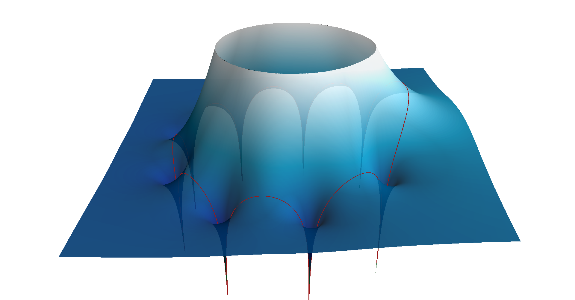$|H(z)|$ surface in the Z-domain. As mentioned above, the DTFT is just a special case of the Z-transform, where $z=e^{i\omega }$, i.e. the unit circle in the complex plane. Remember that the point $z=e^{i\omega }$ is a point with a distance of $1$ to the origin, and with an angle of $\omega \mathrm{rad}$ between its position vector and the positive x axis.

Image source code

The image of the unit circle is shown in red. Notice that this is the same curve as the blue curve in the magnitude response graph above: close to 0 when $\omega \to 0$ (the right half of the circle) and negative when $\omega \to \pi$ (the left half of the circle). The positive x axis points to the right-hand side, the y axis points away from you, and the z axis points up).

Cutoff frequency

The cutoff frequency is defined as the frequency of the half-power point, where the power gain is a half. It's often called the $-3dB$-point, because $10{\log }_{10}\left(\frac{1}{2}\right)\approx -3.01dB$.
To find it, just solve the following equation: $${\left|H\left(e^{i{\omega }_c}\right)\right|}^2=\frac{1}{2}$$ $$\begin{array}{rl}\frac{1}{N^2}\frac{{\sin }^2\left(\frac{{\omega }_{c}N}{2}\right)}{{\sin }^2\left(\frac{{\omega }_c}{2}\right)}& =\frac{1}{2}\\ {\sin }^2\left(\frac{{\omega }_{c}N}{2}\right)& =\frac{N^2}{2}{\sin }^2\left(\frac{{\omega }_c}{2}\right)\\ {\sin }^2\left(\frac{{\omega }_{c}N}{2}\right)-\frac{N^2}{2}{\sin }^2\left(\frac{{\omega }_c}{2}\right)& =0\end{array}$$ This equation doesn't have a general analytical solution, but we can use numerical methods to determine the cut-off frequency. Note that the intersections at zero and $2\pi$ are not valid solutions. In these points the transfer function is undefined, because it evaluates to $0/0$. We only care about the first solution for ${\omega }_c\in (0,\pi )$.
A possible approach to find the intersection is to use the Newton-Raphson method.
A good starting point seems to be at half the period of the high-frequency sine wave.
We don't have to keep the squares, because both sines will be positive in the region of the intersection. $$\begin{array}{rl}f({\omega }_c)& =\sin \left(\frac{{\omega }_{c}N}{2}\right)-\frac{N}{\sqrt{2}}\sin \left(\frac{{\omega }_c}{2}\right)\\ f^{\prime }({\omega }_c)& =\frac{N}{2}\cos \left(\frac{{\omega }_{c}N}{2}\right)-\frac{N}{2\sqrt{2}}\cos \left(\frac{{\omega }_c}{2}\right)\\ {\omega }_c^{(0)}& =\pi /N\end{array}$$ A Python implementation can be found in the get_sma_cutoff function in the snippet below.

Plotting the frequency response, impulse response and step response in Python

We can use the SciPy and Matplotlib modules to plot the frequency response in Python.
This is the script that was used to generate the plots in the previous paragraphs.

from scipy.optimize import newton
from scipy.signal import freqz, dimpulse, dstep
from math import sin, cos, sqrt, pi
import numpy as np
import matplotlib.pyplot as plt

# Function for calculating the cut-off frequency of a moving average filter
def get_sma_cutoff(N, **kwargs):
    func = lambda w: sin(N*w/2) - N/sqrt(2) * sin(w/2)  # |H(e^jω)| = √2/2
    deriv = lambda w: cos(N*w/2) * N/2 - N/sqrt(2) * cos(w/2) / 2  # dfunc/dx
    omega_0 = pi/N  # Starting condition: halfway the first period of sin(Nω/2)
    return newton(func, omega_0, deriv, **kwargs)

# Simple moving average design parameters
f_s = 100
N = 5

# Find the cut-off frequency of the SMA
w_c = get_sma_cutoff(N)
f_c = w_c * f_s / (2 * pi)

# SMA coefficients
b = np.ones(N)
a = np.array([N] + [0]*(N-1))

# Calculate the frequency response
w, h = freqz(b, a, worN=4096)
w *= f_s / (2 * pi)                      # Convert from rad/sample to Hz

# Plot the amplitude response
plt.subplot(2, 1, 1)
plt.suptitle('Bode Plot')
plt.plot(w, 20 * np.log10(abs(h)))       # Convert modulus to dB
plt.ylabel('Magnitude [dB]')
plt.xlim(0, f_s / 2)
plt.ylim(-60, 10)
plt.axvline(f_c, color='red')
plt.axhline(-3.01, linewidth=0.8, color='black', linestyle=':')

# Plot the phase response
plt.subplot(2, 1, 2)
plt.plot(w, 180 * np.angle(h) / pi)      # Convert argument to degrees
plt.xlabel('Frequency [Hz]')
plt.ylabel('Phase [°]')
plt.xlim(0, f_s / 2)
plt.ylim(-180, 90)
plt.yticks([-180, -135, -90, -45, 0, 45, 90])
plt.axvline(f_c, color='red')
plt.show()

# Plot the impulse response
t, y = dimpulse((b, a, 1/f_s), n=2*N)
plt.suptitle('Impulse Response')
_, _, baseline = plt.stem(t, y[0], basefmt='k:')
plt.setp(baseline, 'linewidth', 1)
baseline.set_xdata([0,1])
baseline.set_transform(plt.gca().get_yaxis_transform())
plt.xlabel('Time [seconds]')
plt.ylabel('Output')
plt.xlim(-1/f_s, 2*N/f_s)
plt.yticks([0, 0.5/N, 1.0/N])
plt.show()

# Plot the step response
t, y = dstep((b, a, 1/f_s), n=2*N)
plt.suptitle('Step Response')
_, _, baseline = plt.stem(t, y[0], basefmt='k:')
plt.setp(baseline, 'linewidth', 1)
baseline.set_xdata([0,1])
baseline.set_transform(plt.gca().get_yaxis_transform())
plt.xlabel('Time [seconds]')
plt.ylabel('Output')
plt.xlim(-1/f_s, 2*N/f_s)
plt.yticks([0, 0.2, 0.4, 0.6, 0.8, 1])
plt.show()

Comparing the Simple Moving Average filter to the Exponential Moving Average filter

Using the same Python functions as before, we can plot the responses of the EMA and the SMA on top of each other.
First, the length $N$ of the SMA is chosen, then its $3dB$ cut-off frequency is calculated, and this frequency is then used to design the EMA. Do note that this is a fairly arbitrary decision.

from scipy.optimize import newton
from scipy.signal import freqz, dimpulse, dstep
from math import sin, cos, sqrt, pi
import numpy as np
import matplotlib.pyplot as plt

# Function for calculating the cut-off frequency of a moving average filter
def get_sma_cutoff(N, **kwargs):
    func = lambda w: sin(N*w/2) - N/sqrt(2) * sin(w/2)  # |H(e^jω)| = √2/2
    deriv = lambda w: cos(N*w/2) * N/2 - N/sqrt(2) * cos(w/2) / 2  # dfunc/dx
    omega_0 = pi/N  # Starting condition: halfway the first period of sin(Nω/2)
    return newton(func, omega_0, deriv, **kwargs)

# Simple moving average design parameters
f_s = 360
N = 9

# Find the cut-off frequency of the SMA
w_c = get_sma_cutoff(N)
f_c = w_c * f_s / (2 * pi)

# Calculate the pole location of the EMA with the same cut-off frequency
b = 2 - 2*cos(w_c)
alpha = (-b + sqrt(b**2 + 4*b)) / 2

# SMA & EMA coefficients
b_sma = np.ones(N)
a_sma = np.array([N] + [0]*(N-1))

b_ema = np.array((alpha, 0))
a_ema = np.array((1, alpha - 1))

# Calculate the frequency response
w, h_sma = freqz(b_sma, a_sma, worN=4096)
w, h_ema = freqz(b_ema, a_ema, w)
w *= f_s / (2 * pi)                      # Convert from rad/sample to Hz

# Plot the amplitude response
plt.subplot(2, 1, 1)
plt.suptitle('Bode Plot')
plt.plot(w, 20 * np.log10(abs(h_sma)),   # Convert modulus to dB
         color='blue', label='SMA')
plt.plot(w, 20 * np.log10(abs(h_ema)),
         color='green', label='EMA')
plt.ylabel('Magnitude [dB]')
plt.xlim(0, f_s / 2)
plt.ylim(-60, 10)
plt.axvline(f_c, color='red')
plt.axhline(-3.01, linewidth=0.8, color='black', linestyle=':')
plt.legend()

# Plot the phase response
plt.subplot(2, 1, 2)
plt.plot(w, 180 * np.angle(h_sma) / pi,  # Convert argument to degrees
         color='blue')
plt.plot(w, 180 * np.angle(h_ema) / pi,
         color='green')
plt.xlabel('Frequency [Hz]')
plt.ylabel('Phase [°]')
plt.xlim(0, f_s / 2)
plt.ylim(-180, 90)
plt.yticks([-180, -135, -90, -45, 0, 45, 90])
plt.axvline(f_c, color='red')
plt.show()

# Plot the impulse response
t, y_sma = dimpulse((b_sma, a_sma, 1/f_s), n=2*N)
t, y_ema = dimpulse((b_ema, a_ema, 1/f_s), n=2*N)
plt.suptitle('Impulse Response')
plt.plot(t, y_sma[0], 'o-',
         color='blue', label='SMA')
plt.plot(t, y_ema[0], 'o-',
         color='green', label='EMA')
plt.xlabel('Time [seconds]')
plt.ylabel('Output')
plt.xlim(-1/f_s, 2*N/f_s)
plt.legend()
plt.show()

# Plot the step response
t, y_sma = dstep((b_sma, a_sma, 1/f_s), n=2*N)
t, y_ema = dstep((b_ema, a_ema, 1/f_s), n=2*N)
plt.suptitle('Step Response')
plt.plot(t, y_sma[0], 'o-',
         color='blue', label='SMA')
plt.plot(t, y_ema[0], 'o-',
         color='green', label='EMA')
plt.xlabel('Time [seconds]')
plt.ylabel('Output')
plt.xlim(-1/f_s, 2*N/f_s)
plt.legend()
plt.show()